Data Vis

Author

Shifa Maqsood

#Data types

There are different data types in R: numeric, character, and logical

Numeric data

It has two type: integer and double

Integers do not have decimal point and double do.

numeric_data <-c(10.4,7,4) #DOUBLE
typeof(numeric_data[1])
[1] "double"
typeof(numeric_data[2])
[1] "double"
typeof(numeric_data[3])
[1] "double"
is.numeric(numeric_data[3]) #to check the data type. retuns false or true
[1] TRUE
typeof(7L)
[1] "integer"

Character data

Characters are also called strings. Anything between quotation marks “” is treated as character

typeof("what is the date today?") #tells the type of data
[1] "character"
my_string <- "The instructor said, \"R is cool,\" and the class agreed."
cat(my_string) # cat() prints the arguments
The instructor said, "R is cool," and the class agreed.

Logical

x<- c(4,5,6,7) #this one asks if 7 is found in the object x
 7 %in% x 
[1] TRUE
class(TRUE) #it tells that the class of true is logical
[1] "logical"

Factor data

When you use factor, you are telling R that this is categorical data with levels. This can be very helpful in various types of statistical analysis.

myfactor <- factor("B", levels = c("A", "B","C")) # B is a factor which has three levels A,B and C
myfactor 
[1] B
Levels: A B C

#Tidy data

Untidy data can be hard for us and the computer to read and do anlaysis on it. In tidy data, every column is variable, every row is an observation and every cell is a single value.

untidy_data <- read.csv("CopyOfdata/untidy_data.csv")


untidy_data
  customer_id itemsprice_2018 itemsprice_2019 itemsprice_2020 totalprice_2018
1           1        2 (3.91)        8 (4.72)       10 (5.59)            7.82
2           2        1 (3.91)        6 (4.72)        1 (5.59)            3.91
3           3        4 (3.91)        5 (4.72)        5 (5.59)           15.64
4           4       10 (3.91)        1 (4.72)        3 (5.59)           39.10
5           5        3 (3.91)        9 (4.72)        8 (5.59)           11.73
  totalprice_2019 totalprice_2020
1           37.76           55.90
2           28.32            5.59
3           23.60           27.95
4            4.72           16.77
5           42.48           44.72
#This is an example of untidy data. 
#It shows that itemprice has two values in each cell
#It is hard to read as it shows the data for all three years repeatedly which can be confusing to analyze.
tidy_data <- read.csv("CopyOfdata/tidy_data.csv")

tidy_data #This is an example of tidy data. It shows how each observatio ihas its own row and each value has its own cell.
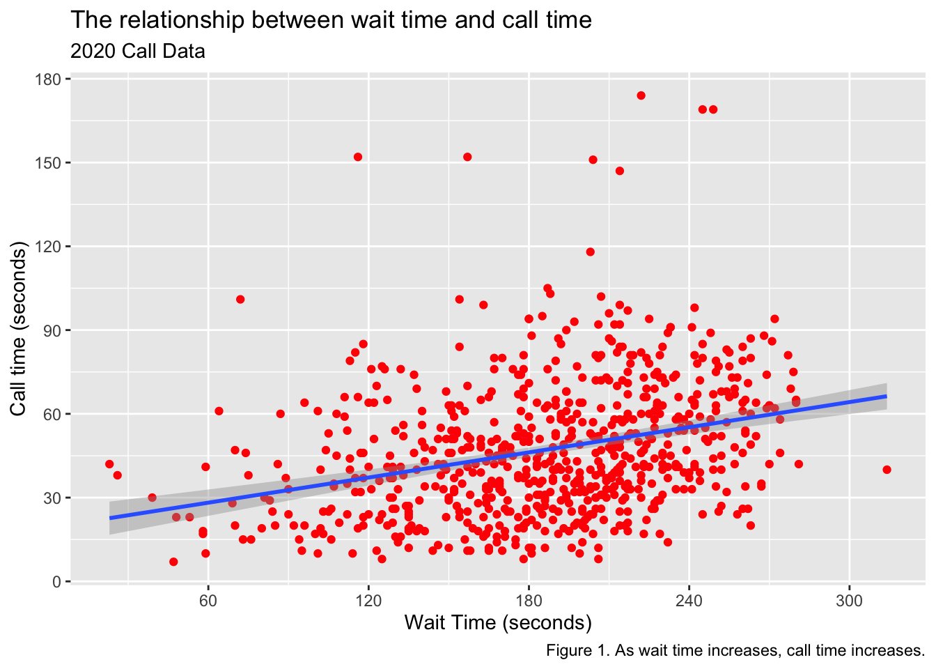
   customer_id year items price_per_item totalprice
1            1 2018     2           3.91       7.82
2            1 2019     8           4.72      37.76
3            1 2020    10           5.59      55.90
4            2 2018     1           3.91       3.91
5            2 2019     6           4.72      28.32
6            2 2020     1           5.59       5.59
7            3 2018     4           3.91      15.64
8            3 2019     5           4.72      23.60
9            3 2020     5           5.59      27.95
10           4 2018    10           3.91      39.10
11           4 2019     1           4.72       4.72
12           4 2020     3           5.59      16.77
13           5 2018     3           3.91      11.73
14           5 2019     9           4.72      42.48
15           5 2020     8           5.59      44.72

#GGplot

library(ggplot2)

survey_data <- read.csv("https://psyteachr.github.io/ads-v2/data/survey_data.csv")

survey_ggplot <- ggplot(survey_data, aes(x = wait_time, y = call_time)) +
  geom_point(colour= "red") +
  geom_smooth(method =lm) + 
  
  scale_x_continuous(name = "Wait Time (seconds)",
                     breaks = seq(from=0, to= 600, by=60))+
  
  scale_y_continuous(name = "Call time (seconds)",
                     breaks = seq(from = 0, to = 600, by = 30))+
  labs(title = "The relationship between wait time and call time",
       subtitle = "2020 Call Data",
       caption = "Figure 1. As wait time increases, call time increases.")


survey_ggplot
`geom_smooth()` using formula = 'y ~ x'